Need for speeds

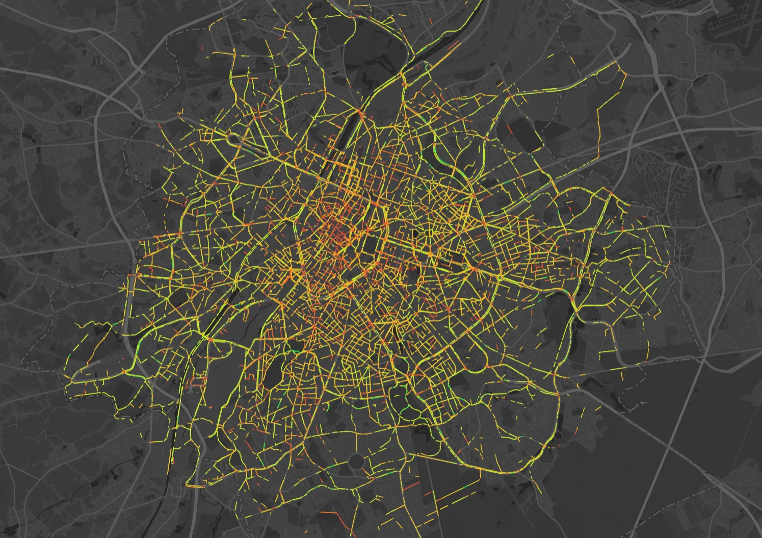
Heat map visualisation of Urbike fleet GPS traces displaying average cycling speeds across the urban network.
The delivery optimisation challenge
If you want to optimise how to deliver things, you need to know how long each delivery will take. Conveniently Google has an API for that! Unfortunately running a single optimisation requires us to know all possible delivery times, so for 10 tasks 10 × 10 = 100 routes. That does not scale well: 100 tasks means more than 10,000 routes (or $5 list pricing) per optimisation, which quickly gets too expensive for the lean budget of a small startup.
One easy solution is to pretend that couriers move in a straight* line at a fixed speed. It is well-known, that in general couriers tend to move around walls and can not fly so these estimates turn out to be a tad optimistic (unless your couriers can go through walls in which case carry on).
* Typically great-circle distance using the Haversine formula.Enter the routing engine
Fortunately, I’ve spent more time thinking about various implementations of Dijkstra’s algorithm than would be healthy for any human being. What we need is a routing engine! Given some start and end locations, the routing engine will provide us with an estimate of how long it would take to cycle from the start to the destination. It does so by what is known as solving the “Shortest-path Problem”. But don’t be deceived, we are not optimising for distance, but for duration – roughly. Actually, what we’re really optimising is a calculated ‘cost’ metric that combines various factors like distance, road type, and number of turns. We then pray this theoretical optimisation translates into genuinely faster routes in real-world conditions.
The basic input to such a system is the street network that we model as a graph. The costs for each edge translate to the time it takes to travel over a certain street plus some of the aforementioned Voodoo. How does the routing engine know how long it’ll take to travel over a certain street? Well it doesn’t, we have to somehow tell it how to do that.
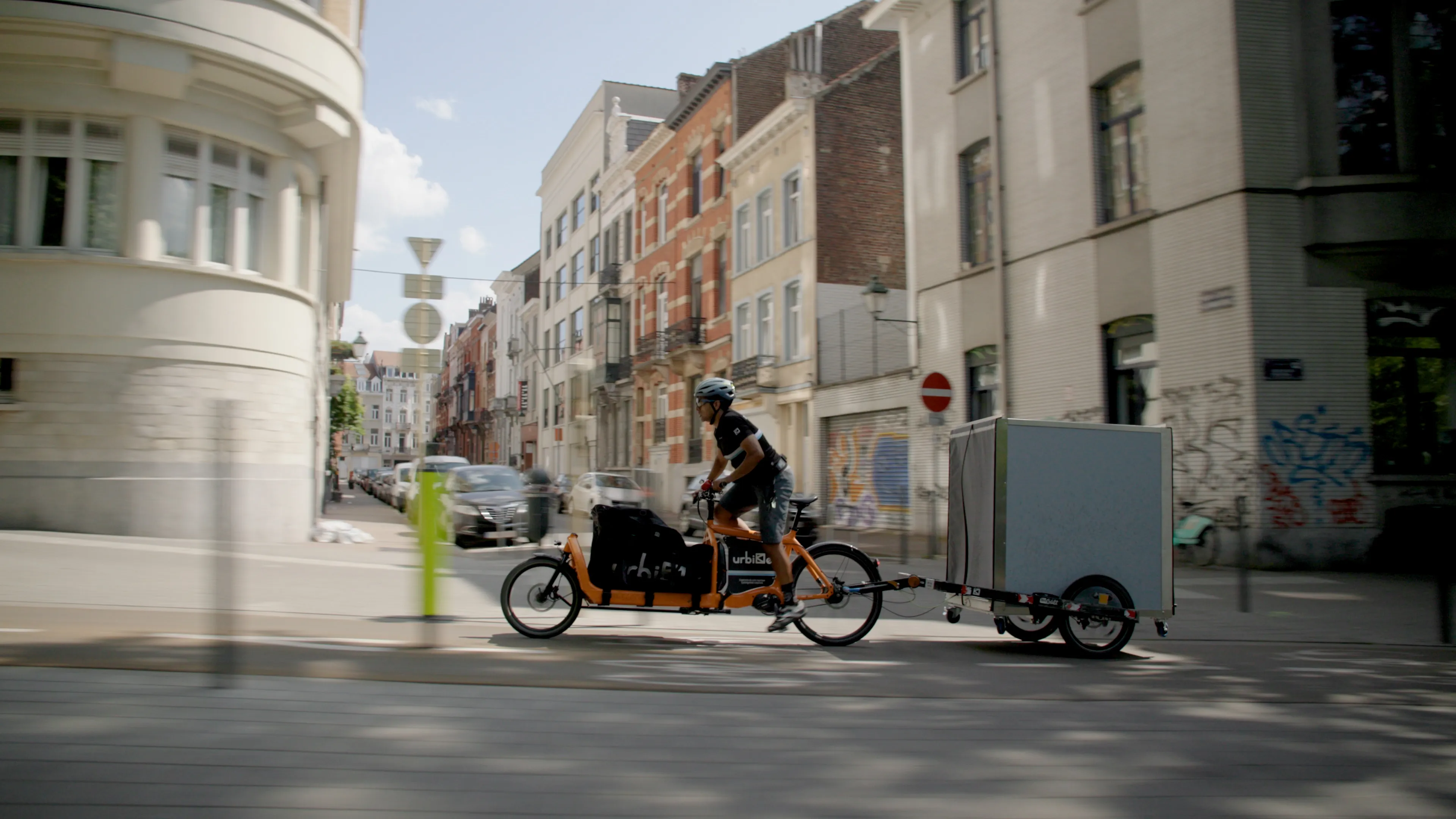
Urbike cargo bikes making deliveries in the centre of Brussels.
Building routing for e-cargo bikes
In most cases, we solve this by guessing the speed based on various features like the road class, the speed limit, urban vs. rural. Since cities tend to be somewhat congested this usually generates really optimistic estimates. We could spend a big bag of money and buy ourselves some actual speed data from established traffic data providers to get real-time and average speeds for most major streets. Since most of our customers are using e-bikes or cargo bikes that wouldn’t be a good way to spend our money though: Their top speed is usually 25 km/h which is lower than most cars, but they are also small enough to weave through traffic or can use dedicated bicycle lanes/streets that bypass car congestion entirely.
Since e-bikes are theft-prone, operators tend to track their fleets with GPS trackers, which gives us a valuable source of GPS data that’s already being collected. Raw GPS data in urban environments is notoriously noisy, and we can’t rely on the filtering usually applied in most mobile operating systems since our data comes from basic onboard devices. The tracking is also intentionally sparse to preserve battery life.
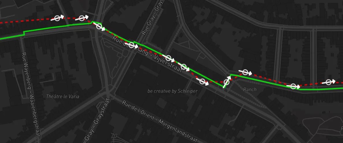
If you have sparse, noisy GPS data and want to figure out which part of a graph was actually traversed, you can use an approach called Map Matching. Ten years ago I wrote this in-depth blog post about it, so I won’t go too much into detail here on how that works. Below is an example of a GPS trace in red and its map-matched counterpart in green:
From raw GPS data to speed models
Thanks to map matching, for each pair of GPS locations and their timestamps, we know which streets in our graph were traversed. So travel distance divided by time, pronto we have the average speed over those segments of the graph. Rinse and repeat for a few gazillion traces and boom we have our own artisan hand-crafted cargo bike speeds.
This gives us a nice dataset of speeds, but it is only accurate where we have seen a significant amount of data. What we want to improve though is not only the speeds where we have data, but also the heuristics we use to derive speeds where we don’t have actual measurements yet.
When it comes to how fast you can cycle, there is one factor every cyclist is painfully aware of: the surface of the street. Going over some rough cobblestones is a very different experience than going over smooth asphalt. So one question we can ask with this data is: Given the surface makeup of the matched streets, what was the actual average speed for each individual surface?
Every pair of trace points is one measurement of an average speed over multiple street segments with different surfaces. For example, we know that the average speed of a bunch of segments was 17 km/h and they consist of 50% asphalt, 20% cobblestone, and 30% dirt. How do we know what the speed on each surface was? We can’t derive this directly, but given we have lots of measurements we can try to find speeds that work well for most measurements we have. Given we are working with speeds here, we can not simply use a linear formula like:
average speed = 50% asphalt speed
              + 20% cobblestone speed
              + 30% dirt speed
But instead need to use the harmonic mean:
average speed = 1 ÷ ( 50% ÷ asphalt speed
                    + 20% ÷ cobblestone speed
                    + 30% ÷ dirt speed )
You can either transform this into a different linear form and solve it directly as a linear regression or just feed it directly into an optimisation system that can natively handle cost functions with non-linear terms. Do this with enough correlated features and you will need to find yourself an ML Engineer.
That being said, the variance in the mean and distribution of speeds for the same surface can still be large. To illustrate this we overlaid the speed histogram of multiple segments of the same surface type (each a different colour).
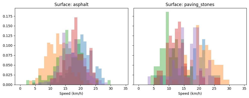
So it pays off to build a robust segment-level dataset over time and learn the precise speeds depending on the environment and the operation of our customers. The differences can be substantial – for example, ground surface averages only 8km/h while asphalt allows for speeds up to 19km/h. Even sett (“Belgian blocks”) significantly impacts speed, reducing it by 30% compared to asphalt. These variations have major implications for route optimisation.
Real-world validation
To validate our approach, we compared our specialised routing engine against industry standards. The results demonstrate significant improvements in routing accuracy for cargo bike operations:
- Our specialized routing produces time estimates with a mean net difference of 20% compared to Google’s estimates
- Our average speeds are 18% higher than Google’s predictions, reflecting the reality of cargo e-bike delivery operations
- On average, our routes are more direct, as Google tends to bias heavily toward cycling infrastructure even when it creates large detours
These findings confirm that general-purpose routing engines don’t accurately model cargo bike performance, likely because they don’t account for the specific capabilities of e-cargo bikes (maintaining consistent speeds, navigating through traffic efficiently, etc.).
For delivery operations, these differences translate to significantly more accurate planning and optimisation, allowing for tighter scheduling and more efficient fleet utilisation.
Key findings and implications
In the end, we found a few interesting things when running our analysis for one of our partners in Brussels:
- Surface type is one of the biggest deciding factors in how fast you can go. Fortunately, the OSM community is extremely detail orientated and we have a lot of data about the surface of our routes. This data is valuable even if it seems fairly niche to tag it.
- Bicycle infrastructure doesn’t impact the speed as much as we expected. Dedicated streets for bicycles are usually the fastest, but when it comes to cycle lanes the benefits of an own lane may be eaten up by slower non-e-bike cyclists. In our dataset, only 25% of the travel distance is covered with bicycle infrastructure.
- Unlike with cars, the actual street hierarchy (major street vs. side-street) plays no significant role because there is no speed limit that goes with that. This does not mean they are no differences in their safety but that is not relevant for the speed prediction.
- General-purpose routing engines like Google’s systematically misestimate cargo bike travel times, with our specialised approach showing a 20% mean net difference in duration estimates. This demonstrates the value of purpose-built routing for delivery operations.
- Our direct route selection, avoiding unnecessary detours through cycling infrastructure when faster alternatives exist, better represents how professional cargo bike couriers actually navigate the city.